nato-io-hmm
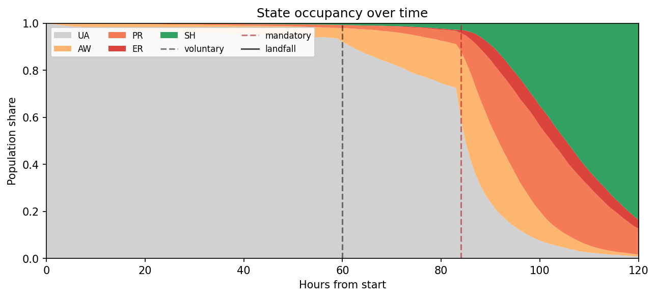
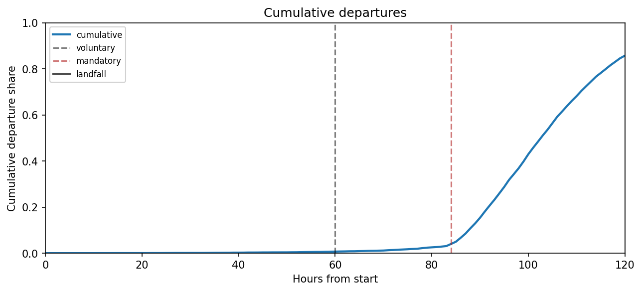
A synthetic hurricane-evacuation household-behavior data-generating process (DGP), designed to be paired with an Input-Output Hidden Markov Model (IO-HMM) fit. The DGP simulates N households over T hourly steps before landfall. Households move through five latent behavioral states (UA → AW → PR → ER → SH) under exogenous forecasts and warning orders, plus two endogenous feedbacks (network congestion, peer-departure share). Three observation channels are emitted each step: a noisy departure indicator, a displacement track, and a communication-activity count.
Pipeline
A single command sequence carries a run from synthesis to bands:
simulate writes a four-file bundle (observations,
population, timeline, config) for one scenario and seed.
fit runs the IO-HMM EM loop with random restarts and
emits its own four-file fit bundle. diagnose recovery
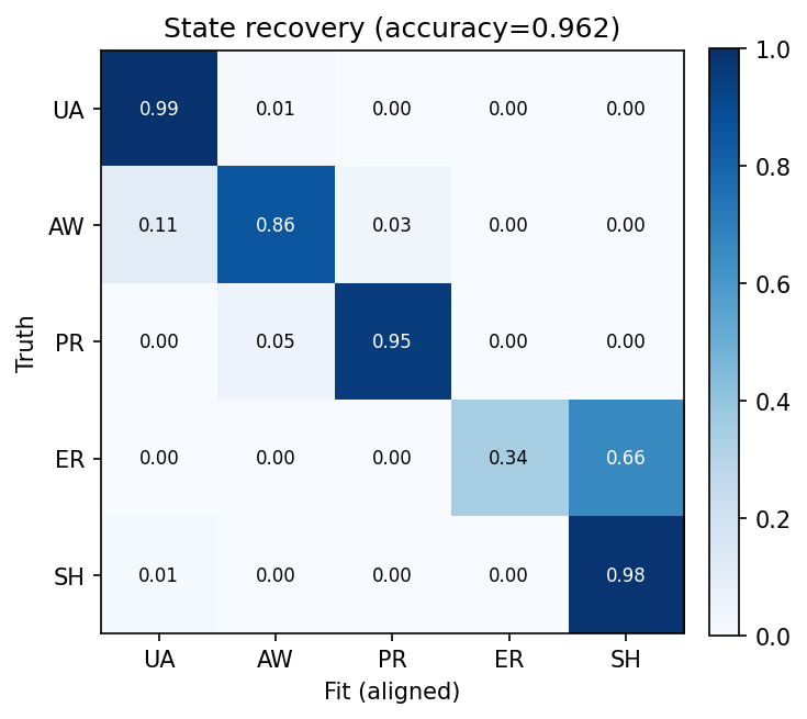
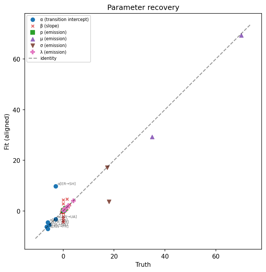
aligns fitted states to truth via the Hungarian algorithm and
writes state- and parameter-recovery metrics. report
renders the smoke-check figures from either bundle.
sweep run repeats the simulation across every
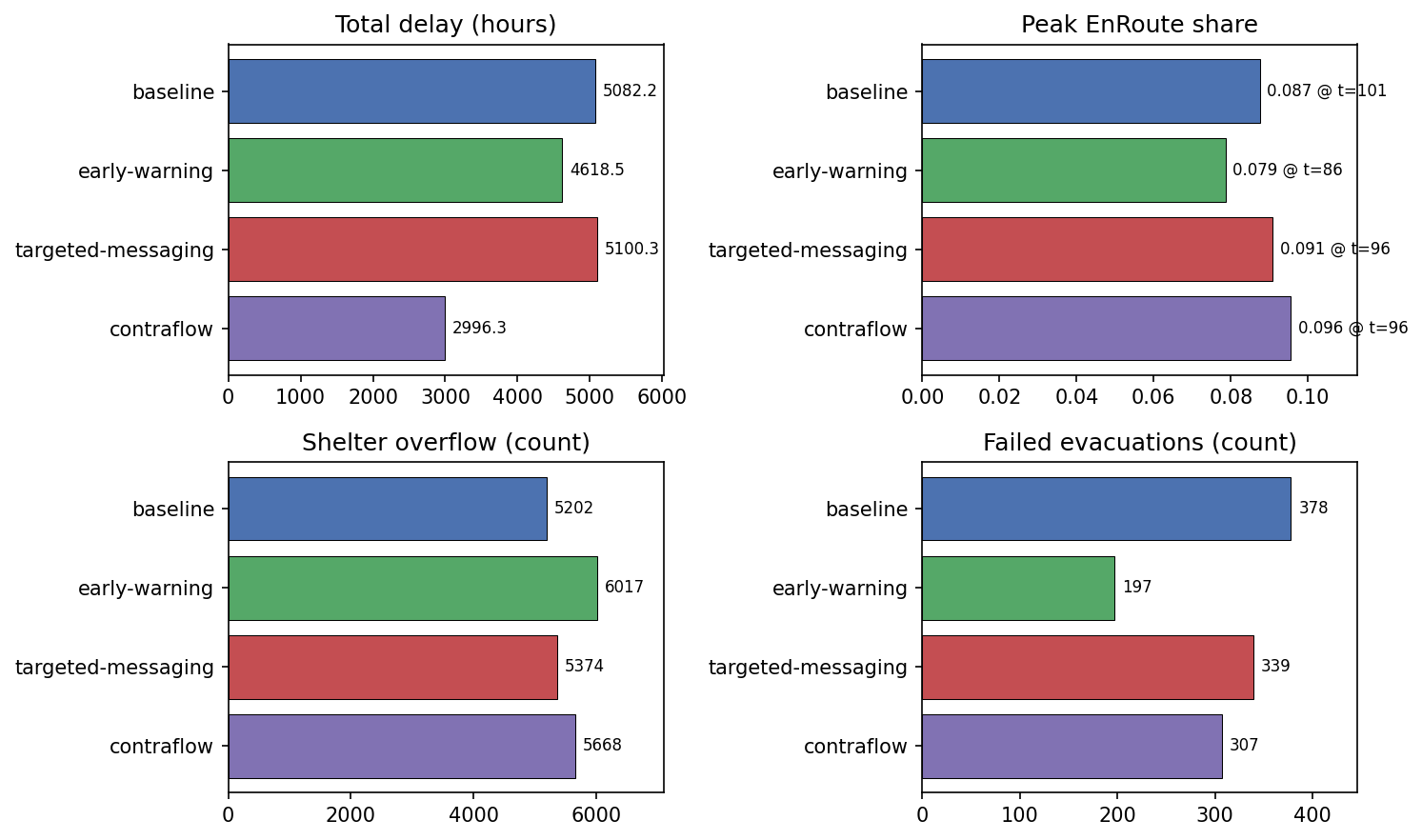
predefined scenario under a common seed; report
sweep-all produces the cross-scenario comparison plots.
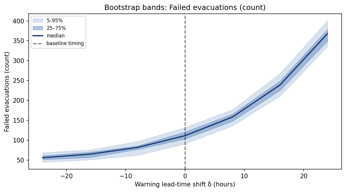
The final stage — bootstrap fit followed by
bootstrap shift-sweep — refits the IO-HMM on
household resamples (joblib parallelism, ~minutes per replicate at
N = 10000) and runs the warning-shift sweep, yielding
quantile bands on failed-evacuation count as a function of
warning timing.
Baseline simulator
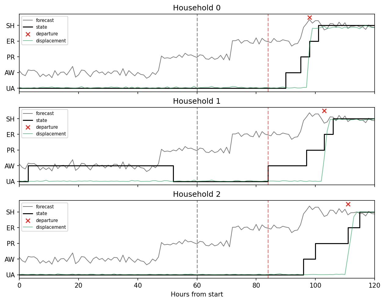
[0, 1, 2]; the CLI
accepts an override.
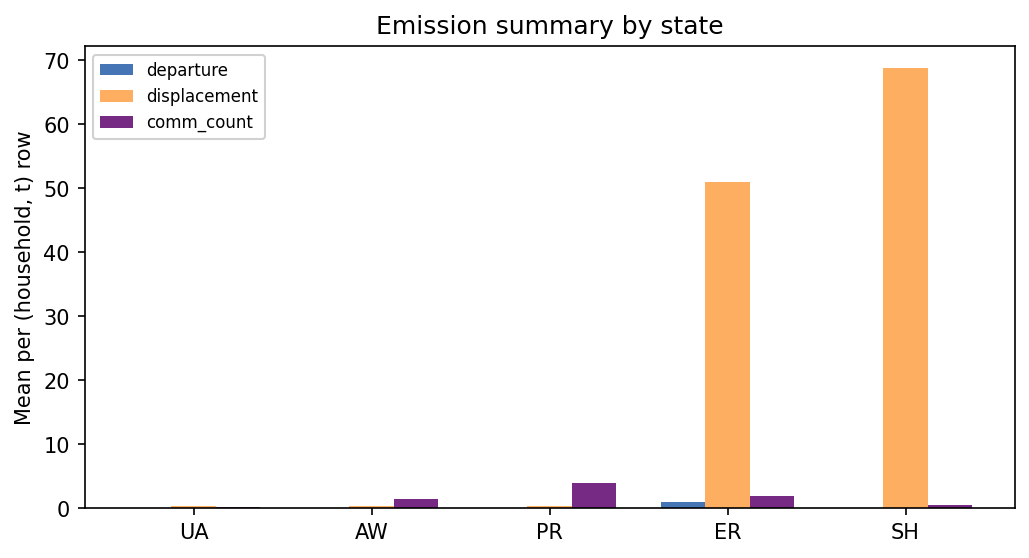
departure, displacement, and
comm_count. Departure mean spikes in ER (~0.95)
and is near zero in UA; displacement is highest in ER and
smaller in SH; communication counts rise from UA through PR
then fall once households are en route or sheltered.
Recovery diagnostics
Scenario sweep
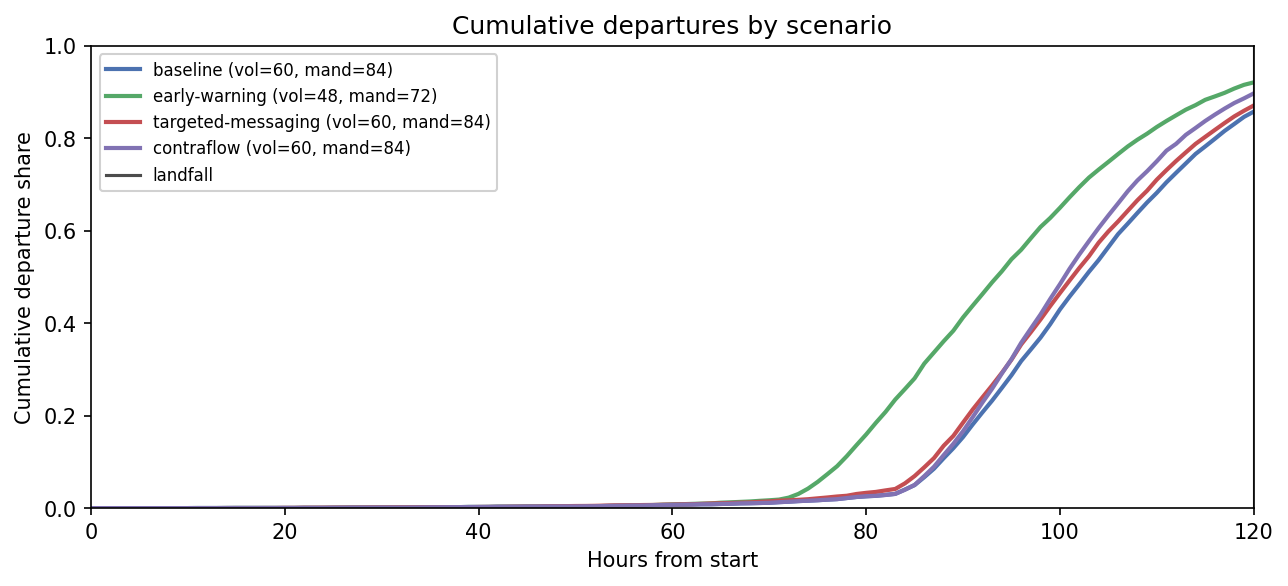
docs/network.md; the figure is the canonical view
of how endogenous network congestion shapes departures
differently from a pure exogenous-forecast model.
Parametric bootstrap
License
AGPL-3.0-only · Copyright © 2026 SWGY, Inc. Distributed without warranty; see LICENSE for the full text.